Explaining models of epidemic spreading
Why do we need Mathematical Models for CoVID-19 ?
In an event like an epidemic, policymakers are keen to know how the disease will spread. For instance, they might be keen to know how many people are likely to be infected in future. This will help them make decisions and allocate resources towards disease control, like the number of ICUs or ventilators required in a region. These and several other predictions concerning the spread of disease are accomplished using mathematical models of epidemiology.
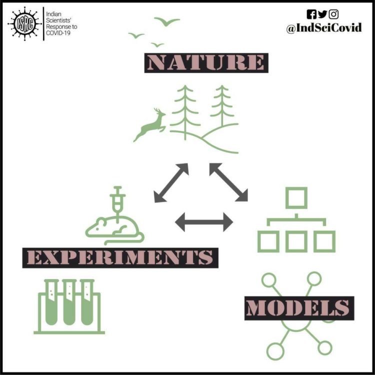
Mathematical models help us make our mental models more quantitative. Models are not reality; however, studies across the natural and physical sciences have shown the importance of models in understanding nature. Say, we need to send a spacecraft to the Moon. To find out how much velocity a spacecraft needs for it to escape the Earth’s gravity, we would not design hundreds of spacecraft and launch them at different speeds to see which one reaches the Moon, right? Instead, we rely on mathematical equations that clearly predict the velocity and all other features that a spacecraft should have, to reach the Moon.
All said, models are not always accurate representations and they do come with limitations. To extend the analogy of the spacecraft designed to reach the Moon, if it were to reach Jupiter, our model would need some tweaks to get it there. It is important to understand the assumptions behind a model and its scope before using it to make predictions and policies.
Models are used to predict the future of the system under study. In the case of epidemics too, we need mathematical modelling to understand how the disease is most likely to spread, and where it is more likely to spread. It can be viewed as a shortcut, instead of implementing many guesses about how to deal with the spread of a disease, we can see what implementing each of these guesses would mean, using some nifty equations, and take more well-informed decisions. Even as you read this, mathematical modelling has been at the heart of several policy decisions worldwide regarding the response to CoVID-19.
Some Aspects of Mathematical Models
So, the question is, how are models developed and used? Typically, models are constructed based on some reasonable hypotheses. For instance, to construct a model for epidemics, one needs to make some assumptions about the mode of disease spread. Measles or Covid19 spread when infected individuals come in contact with healthy ones. Malaria on the other hand needs both mosquitoes and infected humans. A model for malaria would need to take into account the mosquito population as well as that of people and would differ greatly from a model for measles. To give another example of a hypothesis that goes into model formulation, one could postulate age-dependent infectivity, i.e., that the likelihood of being infected on contact, is dependent on the age of the person, with older people more likely to contract the infection. Similarly, one could postulate something about recovery (“younger people recover faster”) or reinfection (“a person who recovers is immune from reinfection for a period of two years”). All these hypotheses can be explicitly incorporated into models. These hypotheses are based on the biology of the disease, i.e., on what we know about the pathogen and the human body. Several different models for the same disease are possible, each differing in the finer details it incorporates among its hypotheses. Needless to say, models are only as good as the assumptions they are based on.
All models have parameters – numbers which can be tuned to suit the particular context to which the model is being applied. For example, consider control measures such as physical distancing. Under normal circumstances, people tend to be physically near each other, leading to a greater likelihood of being infected on proximal contact. When physical distancing is enforced, this likelihood decreases. The likelihood of infection on contact is thus a parameter; when chosen to be small, it captures the situation where physical distancing is being enforced and when chosen large, it captures the business-as-usual scenario. Similarly, age demographics vary by country, state or region. If age-dependent infectivity is part of our model hypothesis, we would need parameters which keep track of the proportion of population in each age-group. These parameters would have markedly different values for India and the US, for example; The Indian population is predominantly young, while that of the US is more evenly spread out across ages. Recovery rates or immunity periods are also parameters, which can be tuned differently to model different diseases. Thus, choosing parameters appropriately allows one to apply the same underlying model to different diseases, different countries or regions, under different control measure scenarios etc.
Once the broad hypotheses and parameters are chosen, the model is written down in terms of mathematical equations. These are typically differential equations, which can then be solved on a computer to obtain the quantities of interest (for eg, the number of infected people) at different points of time.
At the outset, we cannot be sure that we’ve made good choices of parameters. But we correct this slowly by comparing model predictions with actual data (as it becomes available) and tuning our parameters so that there is a close match between these. For instance, if we want to use a new model to predict the number of CoVID-19 infections in Chennai in June 2020, we first validate it using the data on infections until now. In other words, we fit our parameters such that our model is able to explain the daily number of infections until today (April 16, 2020). Once the model is validated, it can be used to predict future behaviour and suggest new experiments to study the population. As days go on and new data becomes available, it is possible to test the model predictions. In some cases, the model is improved/refined as more data becomes available and the cycle continues.
SIR and SEIR Models of Infectious Diseases
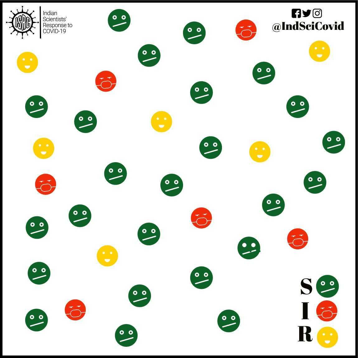
SIR models are commonly used to study the number of people having an infectious disease in a population. The model categorizes each individual in the population into one of the following three groups :
Susceptible (S) – people who have not yet been infected and could potentially catch the infection.
Infectious (I) – people who are currently infected (active cases) and could potentially infect others they come in contact with.
Recovered (R) – people who have recovered (or have died) from the disease and are thereby immune to further infections.
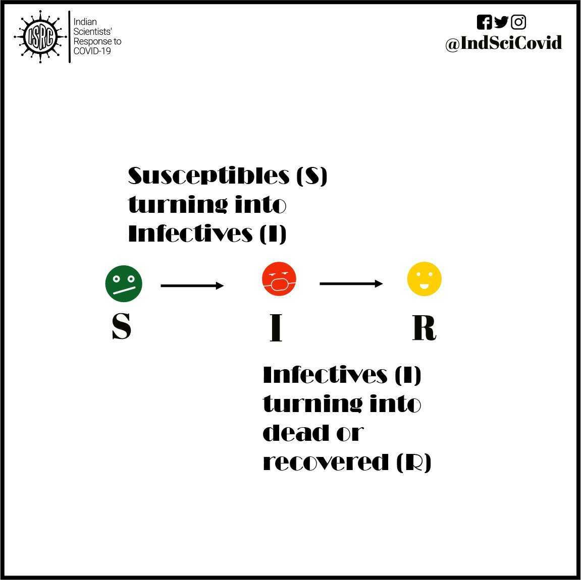
These compartments contain a certain number of people on each day. However, that number changes from day to day, as individuals move from one compartment to another. For instance, individuals in compartment S will move to the compartment I, if they are infected. Similarly, infected people, I will move to the recovered R compartment once they recover or die from the disease.
The total population across the three compartments (S+I+R) is assumed to remain the same at all times. This is just the total population of the country (or state/region) we are considering. This means that everyone exists in one of these 3 compartments. This ignores the fact that in the natural course of things (epidemic or not), births and deaths continue to happen in the country. But for short epidemics that last a few months, this is a reasonable assumption to make! For modelling other diseases like childhood infectious diseases, such as measles, that recur regularly, natural birth and death rates of the population will also have to be taken into account.
As in the current epidemic, from authorized sources such as ministries , one can find the numbers of active cases (I) and the number of recovered or dead (R). Also reported is the total number of infected people to date, which, if one thinks about it, is nothing but the sum I+R.
Our goal is to find out how the number of people in each compartment changes with time. In order to do that, we make two simple hypotheses on what drives the movement of people between these compartments.
The first hypothesis: Let us suppose you have not been infected at this point in time. So, you would belong to the S compartment. You can be exposed to the virus only when you come in contact with an infected person. The greater the number of infected people in the general population, the higher the chance that you will come in contact with an infected individual. This same principle which applies to you, applies equally to every other susceptible individual in the population. Therefore, the rate at which susceptible people become infected, i.e., the rate at which people are transferred from the S to the I compartments on a given day is proportional to the size of the I compartment as well as to the size of the S compartment on that day.
The second hypothesis: Infected people will either recover or die of the disease. On each day, a certain fraction of infected individuals will recover or die. This fraction is taken to be a constant, independent of the number of susceptible, infected, or recovered individuals on that given day. This fraction is somehow “intrinsic” to the specific pathogen and captures the average human body’s recovery time for that particular disease.
What mathematical modellers do is to write the above hypothesis in terms of mathematical equations which tell you how the number of susceptible, infected and recovered individuals change with time. In the language of mathematics, such equations are referred to as differential equations. These equations are solved by a process called integration, and these solutions will allow us to calculate, for example, the number of infected people for any time in future.
For diseases such as CoVID-19, we need to consider another compartment called ‘Exposed’ (E). This consists of individuals who might have the virus (due to travel, direct/indirect with an already positively tested person), but do not show any symptoms. For example, if your cousin travelled to Wuhan and came back she is more susceptible than you – because she has been around the virus. In other words, they are between the susceptible and infected compartments. However, despite not showing any symptoms, these (asymptomatic) individuals can still transmit the disease to susceptible individuals. One can add more compartments, for example, ‘Quarantined’ or ‘Isolated’, to better capture ongoing disease control measures. The modelling proceeds in the same way as in the previous case, with assumptions on the rates at which people move between these compartments. The solution allows us to calculate the number of infectious people at any future time.
Disease Transmission and Containment
Models enable the quantification of the spread of diseases. The rate of spread of infections in a certain population is governed by a quantity R0, called the basic reproduction number. The R0 value can be looked at as the intensity of the infectious disease outbreak. Higher the R0 value of a disease, the faster the disease would spread among the population. In simple terms, the value of R0 is equal to the number of newly infected cases, on average, an infected person will cause. The R0 for measles ranges from 12–18, depending on factors like population density and life expectancy. This shows measles that is a highly infectious disease. If one person gets it, then about 18 will follow. Compared to measles, the novel coronavirus virus is less contagious. As this virus is new, we are not conclusive, but from the evidence we have, R0 ranges from 2.2–2.6. Several biological and social factors come into play in determining the R0. The incubation period, host density, modes of transmission — all affect the R0.

The key insight is if R0 is less than 1, then the epidemic will die out. Thus, our goal is to reduce R0. We can reduce R0 by quarantining contacts of infected people or vaccinating (if a vaccine is available). Another important way to reduce R0, especially for Covid-19, is physical distancing, i.e., maintaining a 1-2 metre distance from other people at all times. Studies show that the novel coronavirus can travel only about a meter in the air as compared to the 100 meters range for an airborne disease like measles. So, physical distancing reduces the probability of picking up an infection. This R0 value, however, is only an average estimate and can be affected by unexpected events such as community gatherings. Here, a single infected person can infect several people and is referred to as a super-spreader. For example, a single infected woman in South Korea attended a church service and ended up infecting 5176 others (as of March 18). This is why public gatherings are forbidden; we do not want to even accidentally trigger the hidden super-spreaders.
Flattening the Curve
In the early stages, the disease spreads rapidly through the population. This is called the exponential growth phase. Here, the total number of infected people (I+R in our SIR model) doubles once every ‘D’ days, where the number ‘D’ for the Covid19 spread in India is around 4 (as of April 6). If this doubling rate continues unabated, the total number of infected people will grow very fast. Even though only a small fraction of those infected will need hospitalisation, our hospitals will reach capacity in a few weeks and cannot serve all those in need of care.
The higher the basic reproduction number R0, the quicker the doubling and the sooner our hospitals will be overwhelmed. If R0 is reduced by control measures (such as physical distancing), then the doubling rate slows down. While very many people will still be infected, this will occur over a longer period of time (months rather than weeks) and the daily demand for hospital beds will not outstrip supply. This stretching out of the infection curve is referred to as flattening the curve.
As days pass by, the number of active infections reaches a peak, after which the spread of infections slows down as fewer and fewer susceptible individuals remain in the population. Mathematical modelling can estimate the number of people who will be infected by the disease at any given time and how this will vary according to control measures imposed. It also gives us an estimate for when the epidemic will peak. In turn, this gives an idea of the number of hospital beds/ICUs required for the population.
Now say, we have a vaccine against an epidemic. This will reduce R0 since the number of susceptibles will decrease. As more people are vaccinated, the disease will come under control. Two Scottish mathematicians, Kermack and McKendrick (who first proposed the SIR model in 1927) showed that we do not have to vaccinate the entire population for an epidemic to die out. Vaccinating only a fraction of the population is enough and this fraction depends on the R0. This fraction for the novel coronavirus causing COVID-19 has been found to be roughly 60%. This result is another example to show how mathematical modelling is extremely useful.
Extensions and Limitations of Models
The compartment models (SIR/SEIR) can be further enhanced using more compartments, such as presymptomatic, asymptomatic, infected-quarantined, infected-recovered, dead, etc. One example is shown below.
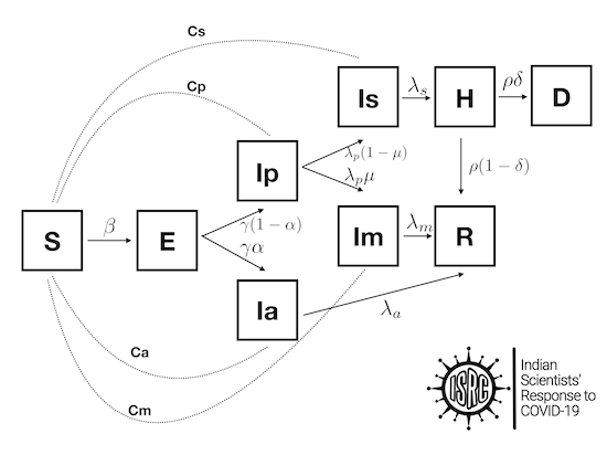
Additionally, people can also be categorized by age, since their response to treatment in the case of COVID-19 is different. Thus, we can construct much richer models starting from the simple SIR model.
However, we notice that to find out the rates at which people from one compartment move to another, we need certain parameters. A model with bad parameters will not yield good results. The more complicated the model, the more there are parameters. These parameters vary with different countries, different regions in different countries. Further, they are affected by various factors such as migrations and non pharmaceutical intervention such as lockdowns, quarantine testing. Obtaining model parameters is a challenge and the general strategy is to look at past behavior and infer the parameters. This procedure, referred to as fitting, is widely used in mathematical modeling. However, these parameters change with time so what was for an earlier time is not valid for a later time.
Since these parameters are reflective of the behavior of humans, they are also affected by perception and information flow. For example, if there is a rumor in a community about a nearby transmission, they will be more conscious about physical interactions. Similarly, messages on various media platforms can change the behavior of people.
In addition to model parameters, the compartment models have a more fundamental limitation as illustrated here. In a SIR/SEIR model, many people fall into the susceptible compartment but not every susceptible individual has the same chance of encountering an infected individual. Healthcare workers, for instance, have more chances of getting infected. Individuals belonging to the same network (social, religious) have varying chances of getting infected depending on their network(s). For example, a shopkeeper meets hundreds of customers a day and therefore his chance of being exposed is much higher. Thus, models that account for individual behavior as opposed to behavior of a collection will capture this variation across individuals in the same compartment. This is where agent-based models (ABMs), also known as individual-based models or IBMs, become useful.
Individual or Agent-based models
Agent-based models (ABMs), also known as individual-based models(IBMs), simulate the behaviour of autonomous agents. While modelling a disease, the agents are usually individual people. This contrasts the previous model which only kept track of how the total number of susceptible, exposed, infectious and recovered patients varies with the progression of time. Thus, the previous model assumes that since each individual acts in a similar way and will have a similar chance of getting infected or transmitting infections. In contrast, ABMs treat each individual separately and their behavior can be different.
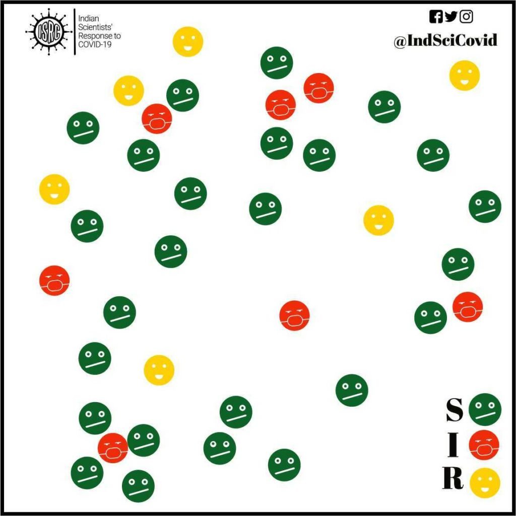
Each agent(individual) has a certain set of properties. The most relevant property is related to their infected state (S, I or R), but there are several other relevant properties. For example, the age, comorbidity, social contacts, etc. vary across individuals and will be relevant factors in the disease spread. Further, there can also be information about the spatial location. At each step(time) of the model, the individuals can change their properties depending on their neighbours. For example, S6 in the figure does not have any neighboring infected agents and will behave differently from S1 which is close to an infected agent. In more advanced models, stochasticity(randomness) and the property of learning from past actions, are incorporated, to reflect more realistic behavior.
ABM simulations, in which individual agents decide what to do in each step, overcomes certain drawbacks of the SIR models and its derivatives, such as the assumption that the population is homogenous. It is possible, for instance, to have different types of agents that represent members of different age groups or of different professions and incorporate facts such as the greater exposure of healthcare workers to infected individuals, which in turn increases their risk of infection. They serve as “bottom-up” models, in which the emergent outcome is determined by the behaviour of the individuals in the population and are more realistic methods of modelling populations. ABMs have previously been used to model diseases at multiple spatial scales, from within a city to across an entire nation. ABMs have successfully been used to model various epidemics including H1N1, various strains of influenza, and Ebola.
One major drawback to ABMs is that as the number of agents increases, so does the computational power required to run the simulation. Large-scale agent-based models tend to require high-performance computing environments for their implementation. Nevertheless, they are the state-of-the-art as far as modeling goes and can be used to model the entire population of a medium-sized city of say 5 million people.
Further Reading:
- Article by Gautam Menon on the modeling of infectious diseases:
https://science.thewire.in/the-sciences/coronavirus-pandemic-infectious-disease-transmission-modelling-kermack-mckendrick-theory-seir-model/ - Article by Vandana RV on the use of mathematics in disease modeling:
https://thefederal.com/the-eighth-column/what-simple-mathematics-can-tell-us-about-coronavirus/ - Article in a set of articles by Bruno Goncalves, NYU on mathematical modeling of diseases https://medium.com/data-for-science/epidemic-modeling-101-or-why-your-covid19-exponential-fits-are-wrong-97aa50c55f8
- Article by Thomas Pueyo describing how different strategies are possible for handling the coronavirus epidemic and how they will lead to different outcomes
https://medium.com/@tomaspueyo/coronavirus-the-hammer-and-the-dance-be9337092b56 - Article by Gautam Menon, ISRC about the some mathematical models that have been proposed recently and their predictive value for India https://science.thewire.in/the-sciences/covid-19-pandemic-infectious-disease-transmission-sir-seir-icmr-indiasim-agent-based-modelling/